Are some languages more efficient than others?
Introduction
Language is a fundamentally human trait that has enabled people to organize into large-scale societies, create works of art that outlast us, and pass on information to new generations. The diversity of human languages is stunning, with thousands of different languages spoken worldwide. They vary in a bunch of ways: how many syllables they use, whether or not they employ tones to convey meaning, syntax, transmission media (e.g. speech, signing), writing systems, and plenty more.
With all this variation, it’s natural to ask whether or not different languages are more or less efficient at communicating information. In a recent new paper titled “Different languages, similar encoding efficiency: Comparable information rates across the human communicative niche” [1], some researchers tackled this exact question using information theory as a framework.
This framework is key to the results, and it’s a fascinating area that touches on so many other scientific fields, so I’ll try to give a quick overview here (feel free to skip if you’re already comfortable). The basic idea is to ground something as abstract as “information” into something a bit more concrete that can then be manipulated mathematically. In this case, as a statistical measure of uncertainty [2]. This perspective shift revolutionized communication technologies by enabling a common language for performance comparisons. It has also provided theoretical insights into noise reduction and upper limits on information compression.
Getting at “information”
A low-information message is one that could be easily guessed. If I told you, “the dog went for a walk in the ___ “ you would probably guess “park” (correct!). Since there’s a strong association between dogs and parks, we might say that the word “park” adds relatively little information to the message. By contrast, if the answer were “volcano” then we would be quite surprised. This is formally measured by a property called entropy, which examines the amount of uncertainty or “surprise” in a message. For any discrete random variable $X$, its entropy is defined as:
\[H(X) = \sum_{i} P(x_{i}) \log_{2} \frac{1}{p(x_{i})}\]So this is just an average! But of what? If we look closer at the $\log$ term, we’ll notice that it’s very small when $x_{i}$ is common, and by contrast really big when $x_{i}$ is rare. This is called self-information and measures our “surprise” about seeing an event $x_{i}$. The base doesn’t really matter but it’s common to use base-2, in which case the resulting measurement is in “bits” [3]. So the entropy $H(x)$ of a random variable measures our average surprise about the variable. It turns out that, for a discrete probability distribution over a finite set of outcomes, this property is maximized with a uniform distribution over events. This kinda makes sense. If we knew that a coin will flip “heads” with probability 1 then a new flip wouldn’t be surprising. By contrast, if heads and tails were equally likely then it’s impossible to predict the upcoming flip any better than chance (at least in the long run). In that sense, a 50/50 split is the one that will surprise us the most on average.
When we think about communicating a discrete set of symbols (hint, hint), then a similar intuition yields. Suppose Bob and Sally write messages to each other in English. Sally writes a word that starts with “q”. What’s the next letter?
Oh, it’s “u”? I’m shocked! Not really of course - that was a very likely outcome so it doesn’t tell us much about the word [4]. We aren’t eliminating very many possibilities by observing this letter.
Study setup
Armed with a grounded notion of “information”, the authors collected audio recordings from participants speaking 17 different languages as well as separate text corpora. The included languages spanned continents and varied heavily, from differing numbers of syllables (several hundred in Japanese, many thousands in English) to the use of tones (0 in most European languages aside from inflections, 6 in Cantonese) to differences in grammatical structure. They then calculated two statistics of interest for each language:
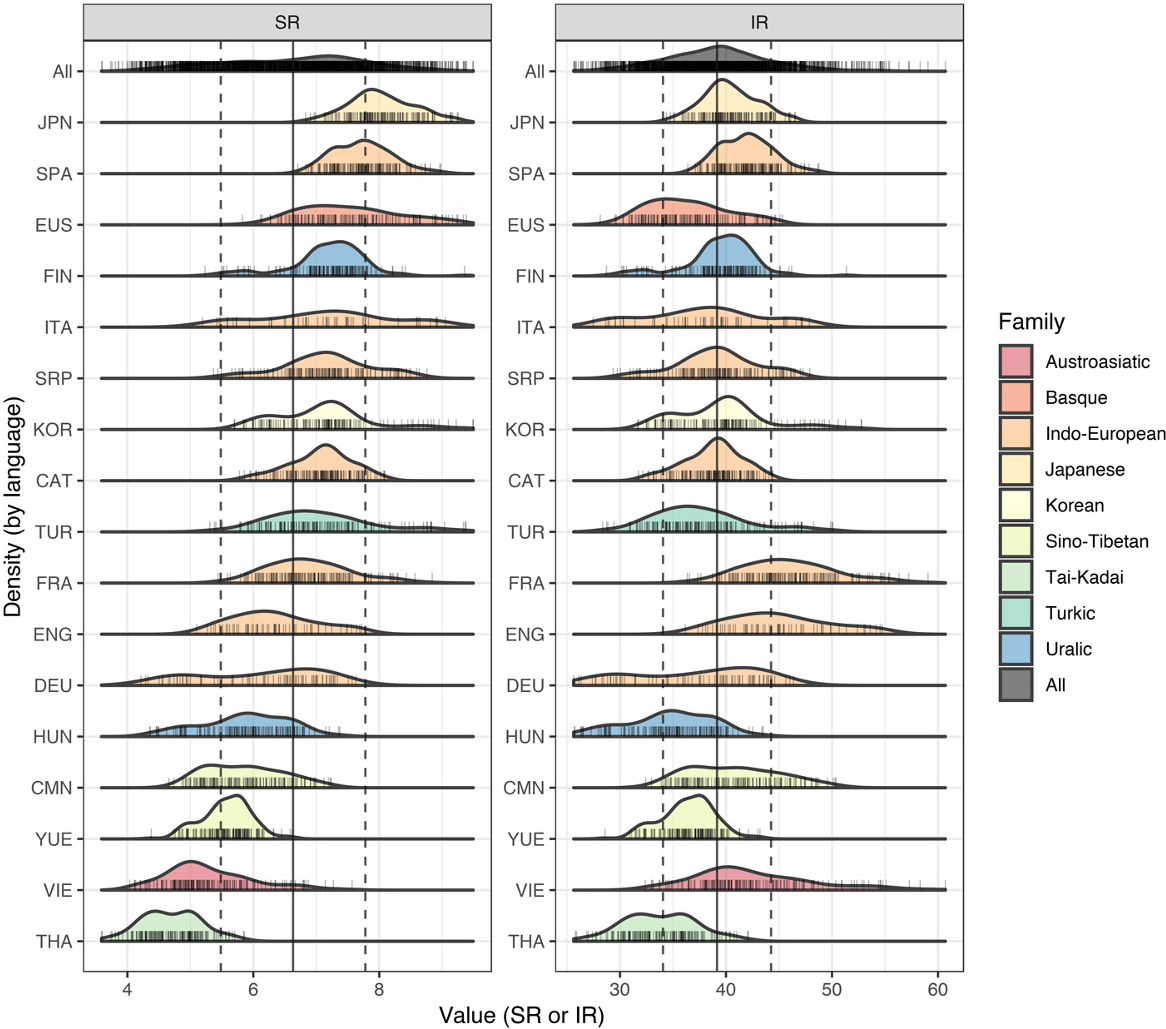
- a syllable rate (SR) measuring the number of syllables/second for an average speaker
- an information density (IR) measuring the extra information in bits gained by each new syllable (we’ll expand on this in a bit)
Using these two values for a given language, the authors then calculated an information rate $IR = SR \times IR$. This resulting value has units of bits/second, and quantifies how much information is transferred on average by a given language.
The participants were asked to read a corpus – a set of writing – in their languages and at their normal speeds. By measuring the number of syllables in those texts and how long it took for each participant, the researchers were then able to determine how fast each language was by calculating a syllable rate (SR) for its speakers. The results showed that languages varied widely in the number of syllables per second, with Japanese having an average SR around eight, while Thai had an average of less than five.
One important note here is that the researchers used the audio text prompts to estimate the number of syllables instead of the spoken audio for each participant. This ignores speaker-specific reductions that simplify words by dropping syllables, such as “probably” –> “prob’bly” in English. On the other hand, the speakers were asked to speak clearly and pronounce sentences fully. The authors also argue that, by focusing on the number of syllables in the corpus, their estimate “emphasize[s] the cross-language comparability of the information encoded and retrievable (i.e., the canonical syllables)”.
With these sentences, they then examined the extra information – reflected by uncertainty – of an upcoming syllable given the previous syllable. This is the information density (ID) from earlier. Let’s mess around with it a bit:
\[\begin{align} ID & = - \sum_{x, y}p(x, y) \log_{2} \big( \frac{p(x, y)}{p(x)} \big) \\ & = - \sum_{x} p(x) \sum_{y} p(y|x) \log_{2} \big( p(y | x) \big) \end{align}\]where we split up the sum and apply Baye’s rule to factorize the joint probability terms. Now we just absorb the negative sign into the $\log$ term and flip it, yielding:
\[= \sum_{x} p(x) \sum_{y} p(y|x) \log_{2} \big( \frac{1}{p(y | x)} \big)\]Cool, this looks easier to grasp! In the inner sum, we’re calculating the average surprise in the upcoming syllable given that we know the current one. With syllables for instance, if “t” only follows “bi” in a language then the “t” has very low information (we could always guess it, so it tells us nothing once it pops up). In the outer sum, we’re doing a weighted average of this value across all pairs of syllables. The entire expression is called the conditional entropy, which we’ll denote as $H(Y | X)$:
\[ID = \sum_{x} p(x) H(Y | X = x) = H( Y| X)\]The resulting ID measures how much new information each consecutive syllable provides, conditioned on the previously uttered syllable. Multiplying this value by the SR (the number of syllables a second), yields the information rate (IR), which measures the amount of information spoken per second.
One might ask: why not condition on more past syllables? Wouldn’t that better reflect how surprised we should be at the current syllable? In short, the authors argue that 1) yes, future followups could do this but 2) their measure is a pretty decent one given that it correlates strongly with yet another meaure of information density which they tried [5]. They also note that they were constrained by some of the text corpora (recall that IDs are estimated from a separate dataset than the oral corpus), which had only word frequencies. I think one other complicating factor might be that you need to calculate $O(k^{n})$ n-gram frequencies for a k-syllable language and a context window of length $k$. That might get difficult fast - on both memory storage and on accurate estimation - but I’m not entirely sure.
Redundancy-efficiency tradeoffs
For all languages in this study, IR values seemed to hover around ~ 40 and subsequent statistical tests showed that languages were much more similar in their IRs than in their SRs. There was also an inverse relationship between IR and SR: languages that had a lot of redundancy (low IR) tended to be spoken more quickly (high SR), and vice-versa. The authors confirmed this through standard correlation measures (Pearson, Spearman correlations) as well as a more involved generalized linear model that adjusted for possible confounders such as age, sex, and the specific text.
Why might this inverse relation exist? The main point is that there is a tradeoff between speed and redundancy. At one extreme, you could have a quick-language-with-too-much-information! In this setting, it could be hard to keep up because of a speaker’s speed and because there’s a lot of information to unpack in what they’re saying. At the other end, a…really…really…slow…and….very…very…redundant…language would be annoying for a listener. Not only is the information you’re getting taking forever, but you’re not learning much either. By optimizing for the overall amount of information transmitted, languages have approached this tradeoff differently. But their IR clustering around a value of ~ 40 suggests an upper limit to information transfer for people. On the speaker’s side, at some point it becomes too difficult to speak quickly and you’ll have to slow down to better pronounce things correctly. On the listener’s side, your cognitive capacity to absorb what’s being said will also hit a ceiling.
In summary, these findings show that diverse languages share a common property, despite the vast differences between them and the physical distances separating their speakers. The results also suggest a fundamental limit on the information processing capacity of the brain, with an upper bound reached despite differences in speech speed and redundancy. On the technology side, I think this work will be helpful in establishing future gold-standard benchmarks for communication prostheses. Rather than measuring performance in something like words/min, which we know will vary across languages, we can shoot for interfaces that provide ~ 40 bits/second.
I think one major question I have about the framework is what sort of gulf divides the lands of “information” (entropy) and “information” (semantics). For instance, context plays a huge role in how messages are interpreted beyond the exact words used. “Bless your heart” can be both a genuine expression or an insult. When quantified as reduction in word/syllable uncertainty, maybe this problem gets smoothed out by conditioning on more prior information (e.g. stress patterns, previous words). But I’m not necessarily convinced that this translates 1-1 with our everyday notion of information (or for that matter if we can even precisely ground it in something concrete).
Footnotes
[1] If the link doesn’t work or it’s paywalled, you can also access the article for free on Scihub :^)
[2] For a great biography on the founder of Information theory, Claude Shannon, I’d recommend “A Mind at Play” by Jimmy Soni and Rob Goodman. The book gives a fun look into Shannon’s quirkiness and personality while also providing great explanations for his work and how they fit into the larger scientific endeavor.
[3] Base-10 is also sometimes used, in which case the units are “Shannons”.
[4] We at least know that it’s not a qindar:
(ˈkɪntɑː ) or qintar (kɪnˈtɑː ) noun plural qindarka (-ˈdɑːkə) or -tarka (-ˈtɑːkə) an Albanian monetary unit worth one hundredth of a lek.
[5] They also tested a “syntagmatic density of information ratio” (SDIR), which is just how much less compression is required to encode the oral corpus relative to some target language (in this case, Vietnamese). The idea here is that the oral corpus texts are semantically similar, so direct comparisons based on syllable length can roughly approximate information density. For a language $L$ with $NS_{t}^{L}$ syllables on oral corpus text $t$ (15 of these in total), its overall SDIR is:
\[SDIR^{L} = \frac{1}{15} \sum_{i=1}^{15} \frac{NS^{VIE}_{i}}{NS_{i}^{L}}\]